Support vector machines
Posted: 08/01/2026
Support vector machines (SVMs) are a set of related supervised learning methods used for classification and regression. They belong to a family of generalized linear classifiers. In another terms, Support Vector Machine (SVM) is a classification and regression prediction tool that uses machine learning theory to maximize predictive accuracy while automatically avoiding over-fit to the data
Hard margin formulation
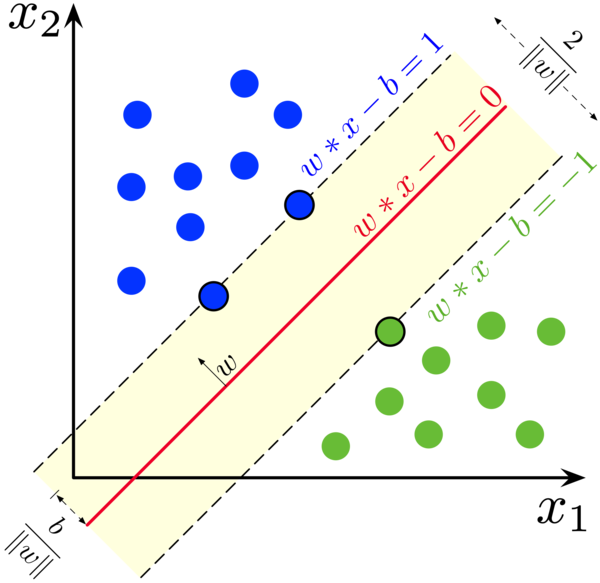
The Support Vector Machine model use an hyperplane \(H\) to compute the predictions with the aim of classifying the data in the correct class. In particular, \(H\) is defined by a vector of parameters \(w=w_1,w_2,...\) and a bias \(b\). In fact, it can be written as
$$ H(x)=\mathbf{w}^T\mathbf{x}+b=w_1x_1+w_2x_2+...+b $$Note that \(\mathbf{y}\) is the vector that contains the labels corresponding to the class of each point. In the simplest formulation of the SVM, the points can be classified only in two different classes, represented by the label \(+1\) for one class and \(-1\) for the other. As a consequence, the vector \(\mathbf{y}\) containing the actual classes is
$$ \mathbf{y}^T=[\pm1,\pm1,...]\Rightarrow y_i=\pm1 $$The margin \(M\) is the distance from the closest point \(x_i\) of the dataset to the hyperplane \(H\). It can be computed as
$$ M(x_i)=\frac{|\mathbf{w}^T\mathbf{x}+b|}{||\mathbf{w}||} $$The support vectors \(\mathbf{x}_{sv}\) are exactly those points on the margin, in other words the points (or point) closest to the hyperplane. To simplify the problem, it is possible to define a new hyperplane \(\bar{H}\), where the new parameters with respect to the previous ones are \(\bar{\mathbf{w}}=\frac{\mathbf{w}} {H(\mathbf{x}_{sv})}\) and \(\bar{b}=\frac{b}{H(\mathbf{x}_{sv})}\). This allows to set the value of \(\bar{H}(\mathbf{x}_{sv})=1\). Note that these steps can be done WLOG (Without loss of generality). Now, the margin can be rewritten as
$$ M(\mathbf{x}_{sv})=\frac{|\bar{\mathbf{w}}^Tx+\bar{b}|}{||\bar{\mathbf{w}}||}=\frac{1}{||\bar{\mathbf{w}}||} $$The idea of the SVM model is to find the hyperplane \(H\) that maximizes the margin \(M\). The objective can function of the optimization problem therefore is
$$ \max_{\mathbf{w},b} M(\mathbf{x}_{sv})\Rightarrow\max_{\mathbf{w},b}\frac{1}{||\mathbf{w}||}\Rightarrow\min_{\mathbf{w},b}||w||\Rightarrow\min_{\mathbf{w},b}||\mathbf{w}||^2 $$Now the constraint. In this basic formulation, misclassification is not allowed, for this reason, the actual class \(y\) and the predicted class \(\bar{y}\) using the hyperplane \(H(x)=\mathbf{w}^T\mathbf{x}+b\) must have the same sign. Note that \(y_i=\pm1\) and \(H(x)\geq1\), because \(H\) was designed to have a minimum value of \(1\) given by the support vectors. The constraint is then
$$ y\cdot\bar{y}\geq1\Rightarrow y\cdot(H(\mathbf{x}))\geq1\Rightarrow y\cdot(\mathbf{w}^T\mathbf{x}+b)\geq1 $$Together, the objective function and the constraint of what is called "Hard Margin SVM" is
$$ \begin{aligned} \min_{\mathbf{w},b} \quad &||\mathbf{w}||^2 \\ \text{s.t.} \quad &y_i\cdot(\mathbf{w}^Tx_i+b)\geq1 \quad \forall i\in \{1,...,n\} \end{aligned} $$The vector of weights \(\mathbf{w}\) and the scalar \(b\) solving the problem are the values that will be used in the classifier \(\mathbf{w}^T\mathbf{x}+b\)
Soft margin formulation
In the "Hard Margin SVM" just described, misclassification was not allowed. However, in real-world dataset, it can happen and it is important to allow a certain amount of it. The first change must be made in the constraint
$$ y_i\cdot(w^Tx_i+b)\geq1-\xi_i $$The \(\xi_i\geq0\) serves as a threshold to allow misclassification, because now \(y\) and \(\bar{y}\) can have different sign. Note that there is a different \(\xi_i\) for each point. However, \(\xi\) must be as small as possible and to reach this goal it is sufficient to add \(\sum\xi_i\) in the objective function which is being minimized. Furthermore, a constant value \(C\) can be added to change the impact of \(\xi\) into the objective function. The final formulation of the "Soft Margin SVM" is
$$ \begin{aligned} \min_{\mathbf{w},b,\xi} \quad &||w||^2 + C\sum_i^N\xi_i \\ \text{s.t.} \quad &y_i\cdot(\mathbf{w}^T\mathbf{x}_i+b)\geq1-\xi_i \\ &\xi_i\geq0 \end{aligned} $$Or, more often, expressed as follows, including \(\frac 1 2\) for simplifing the gradient.
$$ \begin{aligned} \min_{\mathbf{w},b, \xi} \quad &\frac{1}{2}\mathbf{w}^T \mathbf{w} + C\sum_i^N\xi_i \\ \text{s.t.} \quad &y_i\cdot(\mathbf{w}^T\mathbf{x}_i+b)\geq1-\xi_i \\ &\xi_i\geq0 \end{aligned} $$Dual formulation
For a convex optimization problem with inequality constraints
$$ \begin{aligned} \min_{x} \quad &f_0(x) \\ \text{s.t.} \quad &f_i(x)\leq0 \quad i=1,...,m\\ &Ax=b \end{aligned} $$the Lagrangian Dual problem is
$$ \begin{aligned} \max_{\lambda} \quad &g(\lambda, \nu)\\ \text{s.t.} \quad &\lambda_i\geq0 \quad i=1,...,m \end{aligned} $$The function \(g(\lambda,\nu)\) is called Lagrange Dual function and is defined as
$$ \begin{aligned} g(\lambda,\nu) &= \inf_x\bigg(f_0(x)+\sum_{i=1}^m \lambda_i f_i(x) + \sum_{j=1}^p\nu_i(Ax-b)\bigg)\\ &=\inf_x\mathcal{L}(x,\lambda,\nu) \end{aligned} $$Since the Lagrange function can be used as a lower bound for the primal problem, we aim at maximizing it through the Dual Problem. Furthermore, if all the conditions for strong duality holds, a optimal solution of the Dual Problem is also a optimal solution of the Primal Problem. The goal of this section is to derive the Lagrange Dual function in order to write the Lagrange Dual problem that will be used in the solver. Then, the primal variables will be obtained from dual variables.
The KKT conditions of a generic convex problem are
$$ \begin{aligned} \nabla \mathcal{L}(x,\lambda,\nu)=0 &\qquad\text{gradient condition}\\ f_i(x)\leq0 &\qquad\text{primal feasibility}\\ \lambda_i\geq0 &\qquad\text{dual feasibility}\\ \lambda_i f_i(x)=0 &\qquad\text{complementarity condition} \end{aligned} $$Back to the primal formulation of the SVM problem, the Lagrangian \(\mathcal{L}\) can be written as
$$ \begin{aligned} \mathcal{L}(\mathbf{w},b,\xi,\alpha,\beta)= &\frac{1}{2} ||\mathbf{w}||^2 + C\sum_i^m\xi_i \\ &+ \sum_i^m\alpha_i\bigg(-y_i(\mathbf{w}^T\mathbf{x}_i+b)+(1-\xi_i)\bigg) + \sum_i^m\beta_i(-\xi_i) \end{aligned} $$note that \(\alpha_i\geq0\) and \(\beta_i\geq0\) are the Lagrangian multipliers. With the appropriate rearrangements, we write the equalities of the KKT conditions:
$$ \begin{aligned} \mathbf{w}-\sum_{i=1}^n\alpha_i y_i \mathbf{x}_i &= 0\\ -\sum_{i=1}^n\alpha_i y_i &=0\\ C -\alpha_i- \beta_i &= 0\\ \alpha_i(y_i(\mathbf{w}^T\mathbf{x}_i+b)-(1-\xi_i))&=0\\ \beta_i \xi_i &=0 \end{aligned} $$We can use the gradient conditions into the Lagrangian as follows:
$$ \begin{aligned} \mathcal{L} &=-\frac{1}{2}\sum_{i,j}\alpha_i\alpha_j y_i y_j \mathbf{x}_i \mathbf{x}_j + \sum_i\alpha_i \end{aligned} $$For the sake of completeness, we write also the inequalities of the KKT for primal and dual feasibility.
$$ \begin{aligned} y_i\cdot(\mathbf{w}^T\mathbf{x}_i+b)- 1+\xi_i &\geq 0\\ \xi_i &\geq 0\\ \alpha_i &\geq 0\\ \beta_i &\geq 0 \end{aligned} $$Writing \(\beta_i = C - \alpha_i\) with \(\beta_i\geq0\), we can replace \(\beta_i\geq0\) with \(\alpha_i \leq C\). Together with \(\alpha_i\geq0\), we will use the constraint \(0\leq\alpha_i\leq C\). Observe that the stationarity constraint on \(b\) was not used in the calculations for the new objective function, hence it will be added to the Dual Problem as well.
Now, we can write the Dual problem for the SVM problem as \(\max_{\alpha}\mathcal{L}(\alpha)\)
$$ \begin{aligned} \max_{\alpha} \quad &\sum_i\alpha_i -\frac{1}{2}\sum_{i,j}\alpha_i\alpha_j y_i y_j \langle \mathbf{x}_i, \mathbf{x}_j \rangle \\ \text{s.t.} \quad &\sum_{i=1}^ny_i\alpha_i = 0 \\ &0\leq\alpha_i\leq C \end{aligned} $$Although the dual originates from a maximization problem, in practice we will write it as a minimization problem of the negative dual function.
Kernel trick
An important upgrade in SVM classifiers is the use of kernels in the dual formulation. In particular, in the objective function, the dot product \(x_i x_j\), which results in a linear classifier, can be replaced with a nonlinear kernel function \(K(x_i x_j)\).
The result is a more general formulation of the dual:
$$ \begin{aligned} \min_{\alpha} \quad &\frac{1}{2}\sum_{i,j}\alpha_i\alpha_j y_i y_j K(x_i x_j) - \sum_i\alpha_i\\ \text{s.t.} \quad &0\leq\alpha_i\leq C \\ &\sum_{i=1}^ny_i\alpha_i = 0 \end{aligned} $$The four basic kernels are:
- linear: \( K(\mathbf{x}_i, \mathbf{x}_j) = \mathbf{x}_i^T \mathbf{x}_j \).
- polynomial: \( K(\mathbf{x}_i, \mathbf{x}_j) = (\gamma \mathbf{x}_i^T \mathbf{x}_j + r)^d \), \( \gamma > 0 \).
- radial basis function (RBF): \( K(\mathbf{x}_i, \mathbf{x}_j) = \exp(-\gamma \|\mathbf{x}_i - \mathbf{x}_j\|^2) \), \( \gamma > 0 \).
- sigmoid: \( K(\mathbf{x}_i, \mathbf{x}_j) = \tanh(\gamma \mathbf{x}_i^T \mathbf{x}_j + r) \).
Here, \(\gamma\), \(r\), and \(d\) are kernel parameters. This report will be focused on the linear kernel.