Resource Allocation

Posted: 11/07/2025

The Newsvendor Problem

The problems we are going to examine have a forerunner in the Newsvendor Problem, studied as early as 1888. A newspaper seller needs to determine how many newspapers to purchase at the beginning of the day to satisfy the day’s uncertain demand. He faces different costs if he purchases too much or too little:

Too many copies: At the end of the day, some copies are unsold and worthless.
Too few copies: He will sell out and turn away potentially profitable customers.

We name overage cost the cost per unit of purchasing too many items, and underage cost the unit cost of purchasing too few.

If the newsvendor buys newspapers for 20 cents and sells them at 25 cents per unit, then the overage cost is $ O = 20 $ and the underage cost is $ U = 5 $. The overage cost is an actual monetary cost due to a non-optimal decision. The underage cost is virtual, an opportunity cost, i.e. the profit missed due to non-optimal decision (𝑈=25–20).The optimal order quantity is $ y^* $ satisfying

\[ F(y^*) = \frac{U}{U + O} \]

The distribution function $ F(x) $ gives the probability that a probability distribution realizes a value not exceeding the argument $ x $. When we apply the Thompson Sampling algorithm, given a certain instance of Beta distribution, say:

When we apply the Thompson Sampling algorithm, given a certain instance of Beta distribution, say$ \text{Beta}(50, 2000) $ then $ F(0.35) $ is the probability that the new random sample is smaller or equal to 0.35.

The equation above defines the optimal quantity $ y^* $.

The ratio on the right side is:

$ \frac{U}{U + O} = \frac{5}{5 + 20} = 0.2 $

The task is to find the quantity such that with probability less or equal to 20%, the demand will be less or equal to that quantity. Let $ y^* = 0.2 $ Intuitively, buying a copy means betting $20 against $5 that we will resell it. The price balance is 1:4 against us, so the chance balance must be at least 4:1 in our favour, i.e. at least 80%. In other words, the risk of over-buying must not exceed 20%.

The conclusion sounds trivial. But the real problem is to estimate $ F(y^*) $, not to exploit that estimation to find the optimal quantity; that is only the last step. The Newsvendor Problem is a building block to be used in more complex real-life applications.

Capacity Allocation in the Airlines Industry

We are going to treat the Capacity Allocation Problem using as example the airlines industry, where it was initially studied and applied. The example is simplified and voluntarily outdated: nowadays booking systems are much more complex than decades ago, when this problem was initially studied. Not with standing, the concepts we are going to see are still useful as building blocks for complex systems. Similar problems arise in other industries, mainly hotels, car rental and tickets for events.

We are a passenger airline company, selling seats on flights accepting bookings. Our goal is to maximize the revenue:

$ Revenue = Price * Quantity $

where Quantity> is the number of seats sold. We are subject to capacity constraints, e.g. a certain flight has:

$ Capacity = 1000 seats $

In order to maximize revenue, we can use both levers, Price and Quantity. Here we use only Quantity, assuming Price as already assigned. For this reason, the problem is named Capacity Allocation.

The idea is to divide the available capacity in two or more blocks, allocating each block to a different segment. The marketing term Segmentation means splitting the whole population of customers in sub-populations which exhibit:

Similarity inside: customers inside the same segment are "similar“ - each segment is "coherent".
Dissimilarity among: customers of different segments are "dissimilar“ - segments are "differentiated".

Similarity means "with similar behaviors when exposed to similar stimuluses". Intuitively, we mean similar purchasing behaviours.

The Two-Class problem

We start with the following assumptions. Some customers (passengers) are more price-sensitive and accept low prices only, refusing high prices. Less price-sensitive customers prefer low prices (obviously), but if necessary they accept high prices, too. We try to offer the low price to low-spenders and the high price to high-spenders. It is useless to offer the high price to low spenders (they would not buy) and it is counterproductive to offer low price to high spenders (they buy, but we lose the opportunity to sell them at the high price). Unfortunately, it is not so easy to discriminate low and high spenders. We cannot simply interview the masking "Are you available to pay a high-price or a low one only?". High spenders would lie to save money! We need a tool to elicit the true price sensitivity (also called willingness to pay) of each customer. We assume that low-spenders book early, while high-spenders book late. A reasonable justification is that low spenders are mostly leisure travellers, i.e. tourists, while high spenders are mostly business travelers. Yet, what matters here is the correlation between price sensitivity and booking time, not the explanation of the correlation. Indeed, experience supports this hypothesis well enough.

Let us set up a model of our business process of booking policy:

We divide the booking time in two periods.
We fix two prices, $ p_d $ and $ p_f > p_d $, in advance.
In the first period we accept reservations at price $ p_d $, in the second period at price $ p_f $.
The flight has a limited capacity (i.e. number of seats).

Our problem is to find the number of discount booking requests to be accepted at most (the booking limit) and the number of seats to be preserved for full-fare customers (the protection level).

Booking limit $ b $ and protection level $ y $ are bound by the equivalence:

\[ y = C - b \]

where $ C $ is the capacity. So, finding one number means finding the other, too.

Let $ C = 100 $: the flight has 100 seats. If we decide to accept at most 70 requests for discount fare $ p_d $ during the first round of booking, then $ b = 70 $ and consequently $ y = 30 $. Equivalently, we can start reserving 30 seats for the second round, when the fare is $ p_f $. This means to set $ y = 30 $ and consequently $ b = 70 $.

If $ b = 70 $ and in the first round we get 65 bookings, we accept them and we still have 35 seats available in the second round. If in the first round we get 75 bookings, we accept 70 and refuse 5.

The key point is the trade-off between two risks:

Spoiling:
Setting booking limit too low, we will turn away discount passengers requiring a seat in the first round. If in the second round we do not see enough full-fare demand to fill the plane, it will depart with empty seats (spoiled seats).
Dilution:
Setting booking limit too high, we will allow too many customers to book at discount price in the first round. If in the second round we see a full-fare demand exceeding the still available seats, then we will turn away more profitable passengers willing to pay the full fare.

$ P(x) $ = probability of an event

$ d_d $ = demand at discount price $ p_d $, the same for $ d_f $ and $ p_f $

We are reasoning in terms of marginal revenue: the additional revenue brought by an increment of booking limit by one unit.

The question is: what is the additional revenue brought by an increment of the booking limit $ b $?

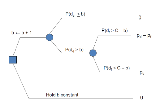
The square node is a decision node: we can choose between incrementing 𝑏 to 𝑏+1 and holding 𝑏 constant. Circle nodes are event nodes: something outside our control happens with a certain probability, and we face some consequences.
The decision of holding 𝑏 constant carries no uncertainty: with probability 1, we gain a marginal revenue of 0. More interesting is the decision of incrementing the booking limit by one more seat:

if there is no request for the added seat, the decision has no real effect; the variation of revenue is 0.
if there is a (𝑏+1)^𝑡ℎ request, then we accept it, while without the increment we would have refused it; we receive an additional 𝑝_d dollars in the first period.
if we have received and accepted the (𝑏+1)^𝑡ℎ request and in the second period the demand trespass the remaining seats, then we must refuse one request and lose 𝑝_f dollars (dilution, opportunity cost, regret).

Let us denote the action of incrementing 𝑏 by one seat with ℎ(𝑏) and the expected value of our decision with 𝐸[ℎ(𝑏)].
Let us define 𝐹_d(𝑥)=𝑃(𝑑_d≤𝑥)
This is the distribution probability function of the demand in the first round. It gives the probability of demand not exceeding 𝑥 bookings. Analogously, 𝐹_f(𝑥)=𝑃(𝑑_f≤𝑥).

The formula for expected marginal revenue of incrementing the booking limit can be written as:

𝐸[ℎ(𝑏)] = 𝐹_d(𝑏) ⋅ 0 + [1 − 𝐹_d(𝑏)] {[1 − 𝐹_f(𝐶 − 𝑏)](𝑝_d − 𝑝_f) + 𝐹_f(𝐶 − 𝑏) ⋅ 𝑝_d}

Simplifying:

𝐸[ℎ(𝑏)] = [1 − 𝐹_d(𝑏)] {𝑝_d − [1 − 𝐹_f(𝐶 − 𝑏)] ⋅ 𝑝_f}

If the term on the right-hand side is greater than zero, then increasing the booking limit we increase the expected revenue.
If it is less than zero, increasing the booking limit we decrease the revenue. Our decision criterion is:

Increase the booking limit from 𝑏 to 𝑏+1 if and only if:

𝐸[ℎ(𝑏)] = [1 − 𝐹_d(𝑏)] {𝑝_d − [1 − 𝐹_f(𝐶 − 𝑏)] ⋅ 𝑝_f} > 0

By definition, [1 − 𝐹_d(𝑏)] cannot be negative, because it is a probability, more precisely the probability of demand in the second round exceeding 𝑏. We can suppress that term and state the decision criterion again:

Increase the booking limit from 𝑏 to 𝑏+1 if and only if:

𝑝_d − [1 − 𝐹_f(𝐶 − 𝑏)] ⋅ 𝑝_f > 0

Rewriting the equation, we get:
Increase the booking limit from 𝑏 to 𝑏+1 if and only if:

1 − 𝐹_f(𝐶 − 𝑏) < 𝑝_d / 𝑝_f

Incrementing the booking limit is a good decision (incrementing expected revenue) if and only if the probability of the demand in the second round exceeding the number of seats left excluded from booking in the first round is less than the ratio between the discount and the full fare.

Note that the ratio on the right-hand side is between 0 and 1, which is consistent with the left-hand side being a probability.

To reach a more intuitive formulation, let us define 1 − 𝐹_f(𝐶 − 𝑏) = 𝑅

The interpretation of 𝑅 is the risk of dilution, i.e., the risk of tomorrow’s regret of having sold the (𝑏+1)^th seat today.

The decision criterion is now:
Increase the booking limit from 𝑏 to 𝑏+1 if and only if: 𝑅 𝑝_f < 𝑝_d

In natural language, we require the certain (probability 1) additional revenue of today, 𝑝_d, to be greater than the possible (probability 𝑅) tomorrow opportunity cost, 𝑝_f.

We are comparing two revenue figures, one certain and one uncertain. Or, if you prefer, we are comparing a revenue figure with a cost figure. In both cases, we are doing an inter-temporal comparison.

Indeed, our decision causes a conflict between our interest today (selling one more seat) and our interest tomorrow (having one more seat available for sale). You can also see it as a conflict between the interest of today-us and the interest of tomorrow-us.

In some sense, this is an auction: the first and the second round are the bidders, and we are the auctioneer assigning the seat to the better bid.

The marginalistic analysis gave us a criterion to choose between incrementing or not incrementing a certain level of booking limit. Now we know how to decide if it is better to hold constant a given 𝑏 or to increment it to 𝑏+1. Using this criterion, we can find the optimal booking limit.

Let us start with booking limit 𝑏 = 0.

Algorithm 1: Marginalistic Analysis.


      1. Initialize b = 0 (starting booking limit)
      2. Set C = capacity (total seats available)
      3. While b < C:
      4.     If 1 - F_f(C - b) < p_d / p_f then
      5.         Increment b by 1
      6.     Else
      7.         Stop loop
      8. End While
      9. b is the optimal booking limit

Or the decision criterion says no. A further increment is not desirable. In both cases, the last level of 𝑏 we reached is the optimal one.

Let us name this last booking limit as 𝑏*.

It is either

𝑏* = 𝐶
or 𝑏* = max 𝑥 such that
$ 1 - F_f(C - x) < \frac{p_d}{p_f} $

We are in the optimal situation if each unitary step in any direction is impossible or makes our situation worse. This intuitive statement is true only if some conditions are satisfied. In many practical problems it is the case. The problem at hand, finding the optimal booking limit, belongs to the class of lucky cases, where these conditions are satisfied.

← Back to Blog List